Fig: Grokking Adversarial Examples. We observe that Deep Neural Networks grok adversarial examples, i.e., obtain delayed robustness, without any special intervention long after test set performance has converged. We present a novel model/data/training agnostic progress measure -- local complexity -- which undergoes a phase change when delayed generalization and/or delayed robustness occurs. We present the training dynamics of robustness and local complexity for a CNN trained on CIFAR10 (left) and a ResNet18 trained on Imagenette (right). We see that during training, complexity around data points increases while the test performance peaks. Following that a phase change occurs resulting in a decline in complexity around the data points; this is when grokking occurs. See paper for CNN-CIFAR100, ResNet-CIFAR10, Transformers-ModAddition and more.

Abstract

Grokking, or delayed generalization, is a phenomenon where generalization in a deep neural network (DNN) occurs long after achieving near zero training error. Previous studies have reported the occurrence of grokking in specific controlled settings, such as DNNs initialized with large-norm parameters or transformers trained on algorithmic datasets. We demonstrate that grokking is actually much more widespread and materializes in a wide range of practical settings, such as training of a convolutional neural network (CNN) on CIFAR10 or a Resnet on Imagenette. We introduce the new concept of delayed robustness , whereby a DNN groks adversarial examples and becomes robust, long after interpolation and/or generalization. We develop an analytical explanation for the emergence of both delayed generalization and delayed robustness based on the local complexity of a DNN's input-output mapping. Our local complexity measure quantifies the density of so-called ``linear regions’’ (aka, spline partition regions) that tile the DNN input space, and serves as a utile progress measure for training. We provide the first evidence that for classification problems, the linear regions undergo a phase transition during training whereafter they migrate away from the training samples (making the DNN mapping smoother there) and towards the decision boundary (making the DNN mapping less smooth there). Grokking occurs post phase transition as a robust partition of the input space emerges thanks to the linearization of the DNN mapping around the training points. Web: \href{https://bit.ly/grok-adversarial}{bit.ly/grok-adversarial}.

A Phase Change in the DNN Partition Geometry Leads to Grokking

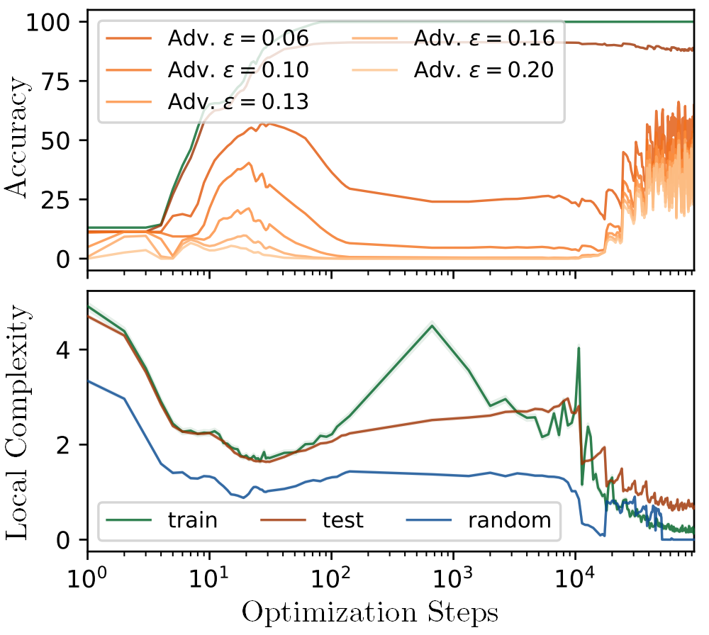
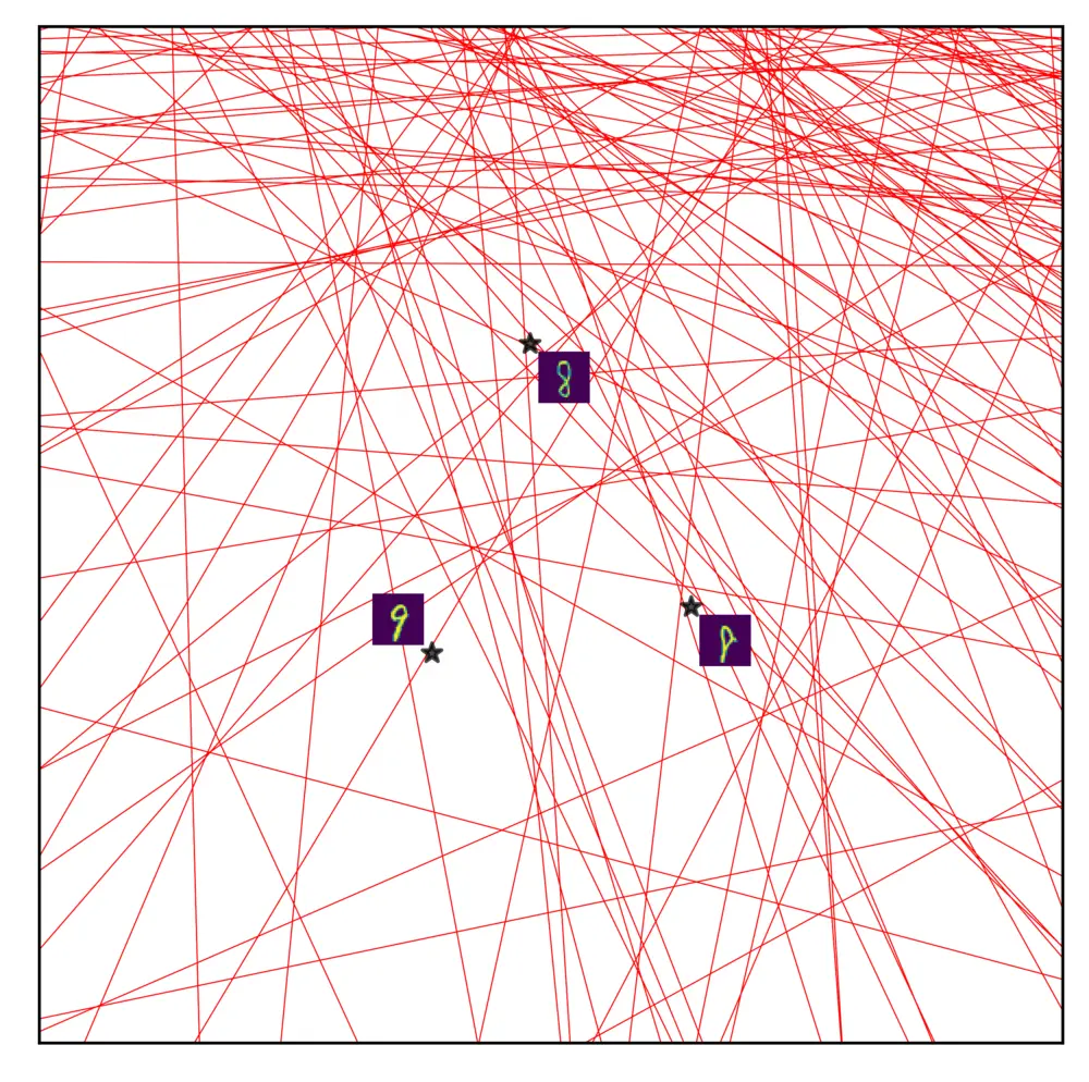
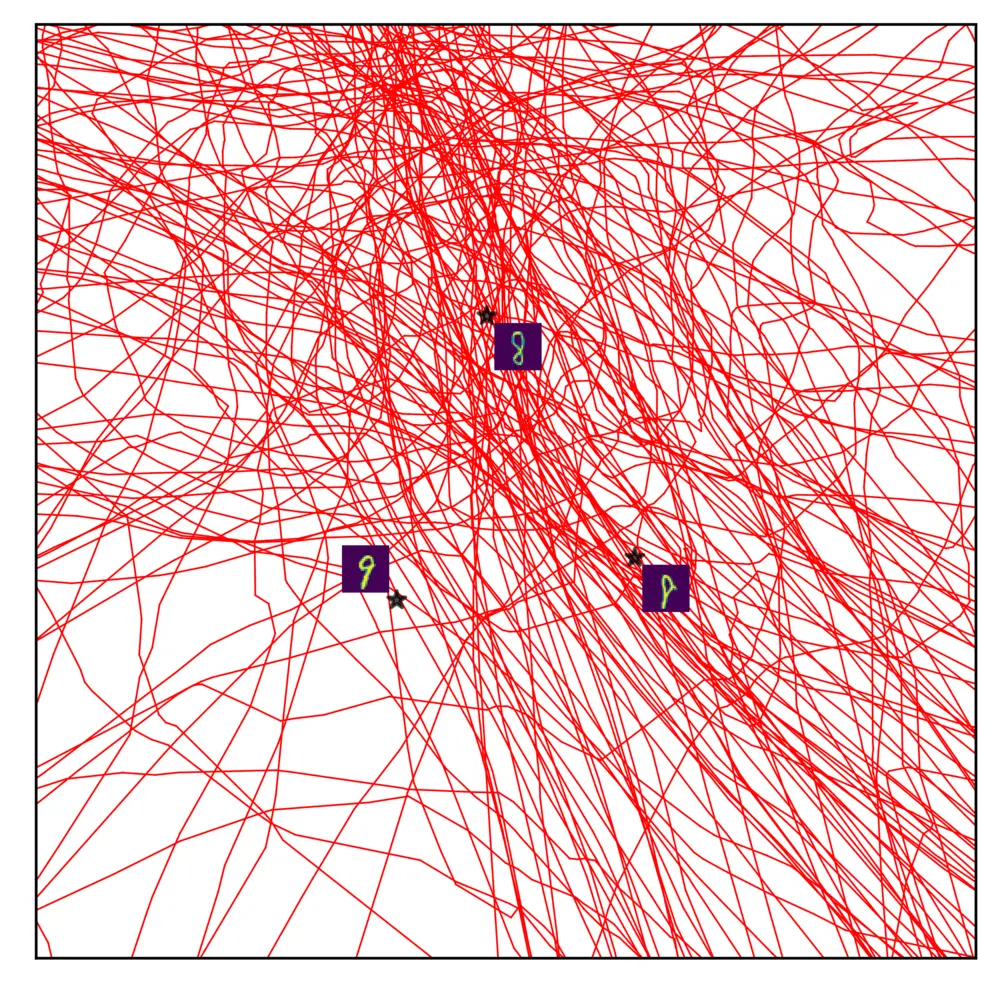
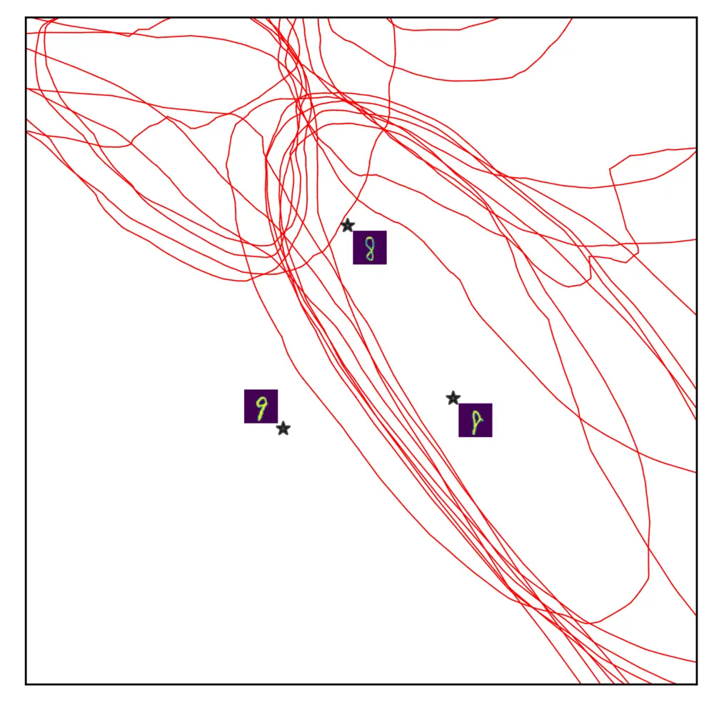
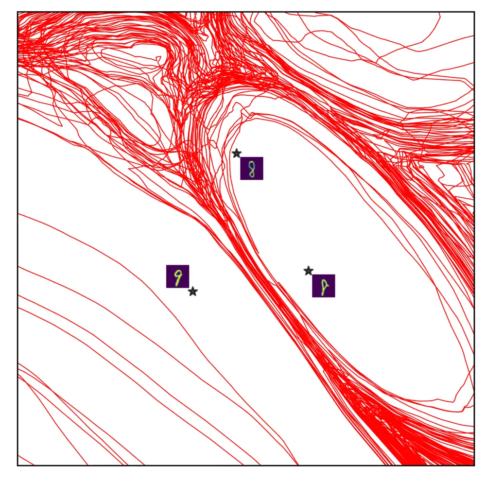
Fig: Grokking Visualized. Every neuron in a DNN learns feature thresholds/boundaries in the input space, dividing it into active and inactive regions. In the video we visualize the analytically computed input space partition formed by the neuron-thresholds (black lines) and decision boundary (red line) of a ReLU-MLP, around three MNIST training samples (white stars). The DNN input-output mapping is linear/affine within each convex region, colored by the norm of the affine slope. In right-top we present the Train, Test and Adversarial accuracy (robustness) and right-bottom we present the local complexity, i.e., density of non-linearities, around training, test and random data points. We see that the network starts grokking adversarial samples as soon as a phase change occurs in the partition (left), also visible in the local complexity (right-bottom), approximately after 10,000 optimization steps.

Accuracy

Train LC

Test LC

Fig: Delayed Generalization. Grokking induced for test samples via large-norm initialization (Liu et al., 2022) for MLPs with varying depth, trained on MNIST. We see that the local complexity (LC) training dynamics is similar to the case of delayed robustness. LC ascents with higher concentration around training samples, following which it descends for training, test and random samples as well. Where do the non-linearities migrate to? We see that during the last phase of training, the non-linearities migrate towards the decision boundary, linearizing the function everywhere else in the process.

Local Complexity - A New Progress Measure

Fig: Linear Regions and Local Complexity. Input space partition formed by a DNN trained to regress the piecewise function defined below (left) and graph of the learned function (right). Each partition region is randomly colored, and performs a single linear operation going from the input to the output. Learned function is more complex, i.e., densely changes the linear operation being performed, where the target function is non-flat.

Progress Measures are defined as scalars that have a causal link with the training state of a DNN. We propose local complexity as a fine-grained progress measure, that at a high level, denotes how complex a DNN input-output mapping is for some local neighborhood in the input space. How can we measure local complexity? DNNs are continuous piecewise affine splines, therefore whenever it is trained to regress a function (could be a classification objective as well), it forms a piecewise linear spline approximation of the target function. For example, suppose we are training an MLP to regress a target function \( f: \mathbb{R}^2 \rightarrow \mathbb{R} \) defined as,

\[ f(x_1, x_2) = \begin{cases} sin(x_1) + cos(x_2) & \text{if } x_1 < 0 \\ 0 & \text{otherwise} \end{cases} \]

Since the function is non-flat only for \( x_1 < 0 \) the DNN assigns more spline knots and forms more 'linear regions' for \( x_1<0 \), just like we would expect in any spline interpolation task. A higher number of linear regions or non-linearities in some input domain, therefore denotes that the learned input-output mapping is more complex within that domain. Through local complexity we can therefore measure how non-linear a function is in some input space locality. For arbitrary dimensional input spaces, local complexity is computed for cross-polytopal input space neighborhoods with a given datapoint as a centroid. During training, these neighborhoods act as probes in the input space where we measure the complexity of the learned function throughout training, therefore monitoring how the non-linearity across different parts of the input space changes.

Fig: Local Complexity Approximation. 1) Given a point in the input space \( x\in \mathbb{R}^D \), we start by sampling \( P \) orthonormal vectors \( \{v_1,v_2,...,v_P\} \) to obtain cross-polytopal frame \( \mathbf{V}_x=\{x \pm r*v_p \forall p\} \) centered on \( x \), where \( r \) is a radius parameter. 2) If any neuron hyperplane intersects the neighborhood \( conv(\mathbf{V}_x) \) then the pre-activation sign will be different for the different vertices. We can therefore count the number neurons for a given layer, which results in sign changes in the pre-activation of \( \mathbf{V}_x \) to quantify local complexity \( x \) for that layer. 3) By embedding \( \mathbf{V}_x \) to the input of the next layer, we can obtain a coarse approximation of the local neighborhood of \( x \) and continue computing local complexity in a layerwise fashion.

Connecting Spline Theory and Mechanistic Interpretability

Fig Interactive: Linear Regions and Circuits. Input space spline partition (left) and network connectivity graph (right) for a randomly initialized 5 layer ReLU-MLP with 5 neurons in each layer, 2D input space, and 1D output space. Neurons are colored blue if active and orange if inactive. Hover and select any of the spline partition regions. Since the input-output mapping is linear per region, the activation/deactivation pattern of neurons remain the same for all vectors from any given region in the input space. This means that each region creates a unique circuit (Olah et al., 2020) comprising of a subset of neurons in the network. The circuit for any two neighboring regions vary by only one neuron being activated/deactivated. This is due to the fact that the knots of the spline partition are the zero level sets of the neurons in the input space. This means that crossing a boundary is equivalent to flipping on or off a neuron in the circuit.

A Circuit is loosely defined as a subgraph of a deep neural network containing neurons (or linear combination of neurons) as nodes, and weights of the network as edges (Olah et al., 2020). It's commonly referred to in mechanistic interpretability literature targeted towards understanding the grokking phenomenon. Since ideally practical DNNs are (or can be approximated as) continuous affine spline operators, for a given piece/region \( \omega \) of the spline, all input vectors \( \{x : x \in \omega\} \), the network performs the same affine operation. The parameters of this affine operation are functions of the activated neurons, meaning that for each region, the network forms a single circuit comprising of only the active neurons. From this perspective, our local complexity measure can be interpreted as a way to measure the density of unique circuits formed in some input space locality. The emergence of a robust partition shows that towards the end of training, the number of unique circuits get drastically reduced. This is especially true for sub-circuits corresponding to the deeper layers. This result, matches with the intuition provided by Nanda et al., 2023 on the cleanup phase of circuit formation late in training.

Layer 1

Layer 2

Layer 3

Layer 4

Layer 5

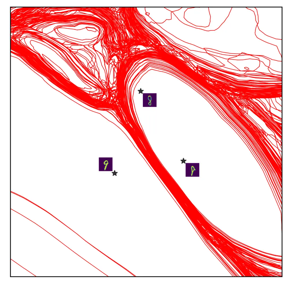
Fig: Layerwise subdivision and circuits. Non-linearities in a DNN accumulates around the decision boundary during grokking, but not equivalently across all layers. This is due to the layerwise sub-division of the spline partition. Deeper layer neurons can be more localized, therefore deeper layers undergo region migration more than shallower layers. Large regions formed in deeper layers would mean deeper layers have more generalized circuits, i.e., the same circuits working for a larger number of data points. In the figure, we show the input space partition in a layerwise fashion, i.e, separately showing the subdivision by each layer.

Citation